



3. More Biases: Survivorship and P-hacking#
The previous two chapters focused on omitted variable bias and sampling bias in detail. Bias, however, takes many more forms. This chapter gives a brief demonstration of two further biases that appear frequently in research. Both section shows a compact, concrete example so you can recognise the pattern in your own work.
Part 1: Survivorship Bias#
What is it?#
Imagine studying what makes a restaurant successful by visiting only restaurants that are still open. Every restaurant in your sample has survived, meaning it already passed some invisible filter. The restaurants that failed (and might have shared many features with your successful ones) simply are not there to be studied. Your conclusions about “success factors” are shaped entirely by that invisible filter.
This is survivorship bias: when your data only contains records of entities that made it through some selection process, while the “non-survivors” are silently excluded. The result is a dataset that looks more successful, more capable, or more extreme than the true underlying population. The survivorship bias is thus a special case of the sampling bias, that arises when the sampling process is influenced by the outcome of interest.
In a wage archive#
Our synthetic dataset simulates a company HR archive. Workers with short tenure and below-median wages are far more likely to have already left as they found better-paying jobs elsewhere or were let go. The archive contains only the workers who stayed. The chart below shows how this filter distorts the distribution of short-tenure employees.
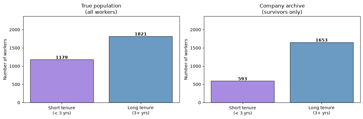
The archive has far fewer short-tenure workers than the true population because most of the low-wage, short-tenure employees have already left. A model trained only on archive data will have rarely seen this group and will get their wages systematically wrong.
feature_cols_s = ['tenure', 'education', 'experience', 'hours_per_week']

# Train the model exclusively on the archive (survivors)
X_archive = df_surv_archive[feature_cols_s].values
y_archive  = df_surv_archive['wage'].values

# Test on the full population including the workers who would have left
X_full = df_surv_full[feature_cols_s].values
y_full = df_surv_full['wage'].values
tenure_full_arr = df_surv_full['tenure'].values

lr_surv = LinearRegression()
lr_surv.fit(X_archive, y_archive)        # learn from survivors only
y_pred_surv = lr_surv.predict(X_full)    # predict for everyone

short_mask_s = tenure_full_arr < 3
long_mask_s  = tenure_full_arr >= 3

print("Model trained on archive (survivors only)")
print("=" * 60)
print(f"  Short tenure (< 3 yrs): RMSE = "
      f"{rmse(y_full[short_mask_s], y_pred_surv[short_mask_s]):.2f} $/hr  "
      f"(n = {short_mask_s.sum()})")
print(f"  Long tenure  (3+ yrs):  RMSE = "
      f"{rmse(y_full[long_mask_s],  y_pred_surv[long_mask_s]):.2f} $/hr  "
      f"(n = {long_mask_s.sum()})")
print()
print("The short-tenure group, mostly absent from training data, has a much")
print("higher error. The model has never seen most of their low-wage records.")
Model trained on archive (survivors only)
============================================================
  Short tenure (< 3 yrs): RMSE = 2.67 $/hr  (n = 1179)
  Long tenure  (3+ yrs):  RMSE = 2.49 $/hr  (n = 1821)

The short-tenure group, mostly absent from training data, has a much
higher error. The model has never seen most of their low-wage records.
Key insight: If you train a model on data that has already passed a selection filter (still-active companies, published studies, surviving projects), the model will perform poorly on the cases that did not survive, often precisely the cases where you most need reliable predictions.
Part 2: P-hacking#
What is it?#
Suppose you want to know whether carrying a lucky charm improves exam results. You test 20 different charms: a rabbit foot, a four-leaf clover, a blue pen, and so on. Even if none of them has any real effect, roughly 1 in 20 tests will appear “statistically significant” just by chance (this is what a significance threshold of 5 % actually means). If you then publish only that one result “blue pens improve exam scores!”, you have committed p-hacking: cherry-picking a significant result from a large pool of tests, while discarding all the non-significant ones.
P-hacking can happen accidentally (a researcher genuinely tests many things and reports the “interesting” result) or deliberately. Either way, it inflates the number of false findings in the scientific literature.
In a wage study#
We generate wages based only on education and experience. Then we invent 20 completely random yes/no attributes for each worker: things like “owns a pet” or “prefers mountains” that have absolutely no relationship to wages. We then test each attribute for a wage effect using a t-test (which asks: “do workers with this attribute earn significantly differently from those without it?”).
# Run a t-test for each random feature: does having it predict higher wages?
# (None of these features have any real effect, they are pure noise.)
p_values = []
for feat in FEATURE_NAMES:
    wages_yes = df_p.loc[df_p[feat] == 1, 'wage']
    wages_no  = df_p.loc[df_p[feat] == 0, 'wage']
    _, p = stats.ttest_ind(wages_yes, wages_no)
    p_values.append(p)

results_p = (pd.DataFrame({'Feature': FEATURE_NAMES, 'p-value': p_values})
               .sort_values('p-value')
               .reset_index(drop=True))

print("T-test results for 20 random features  (none are real wage predictors)")
print("=" * 60)
for _, row in results_p.iterrows():
    flag = "  ← SIGNIFICANT (p < 0.05)" if row['p-value'] < 0.05 else ""
    print(f"  {row['Feature']:<28}: p = {row['p-value']:.3f}{flag}")

n_sig = (results_p['p-value'] < 0.05).sum()
print(f"\n{n_sig} out of 20 tests appear 'significant' at p < 0.05")
print(f"Expected by chance alone: 20 × 0.05 = 1.0")
T-test results for 20 random features  (none are real wage predictors)
============================================================
  Owns a bicycle              : p = 0.024  ← SIGNIFICANT (p < 0.05)
  Born in odd month           : p = 0.091
  Has a tattoo                : p = 0.111
  Prefers tea over coffee     : p = 0.140
  Uses public transport       : p = 0.155
  Plays an instrument         : p = 0.160
  Has siblings                : p = 0.267
  Born on a weekend           : p = 0.321
  Keeps a diary               : p = 0.342
  Reads fiction               : p = 0.380
  Drives to work              : p = 0.381
  First name < 5 letters      : p = 0.439
  Has a middle name           : p = 0.528
  Likes spicy food            : p = 0.534
  Left-handed                 : p = 0.554
  Prefers mountains           : p = 0.583
  Has a garden                : p = 0.628
  Wears glasses               : p = 0.658
  Owns a pet                  : p = 0.819
  Morning person              : p = 0.934

1 out of 20 tests appear 'significant' at p < 0.05
Expected by chance alone: 20 × 0.05 = 1.0
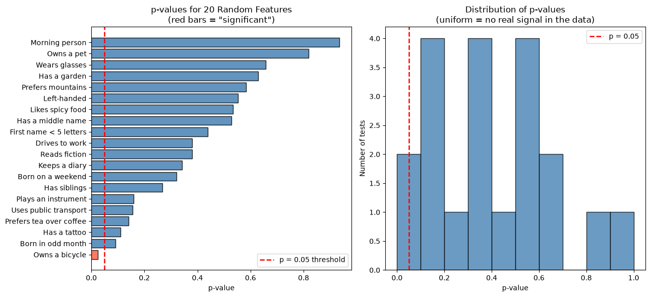
The histogram on the right is the key diagnostic: when there is truly no effect, p-values are spread roughly uniformly between 0 and 1. Only a small cluster at the left edge (below 0.05) represents the “false positives” that chance produces. If a researcher reports only those, the published literature would contain a misleading result about wages.
p-hacking can have many different forms and might happen either accidentally or deliberately. For example:
Researchers might run non-deterministic algorithms (like random forests) multiple times and report only the best result.
They might test many different model specifications (adding or removing features) and report only the one that yields a significant result.
They might also consider certain data points “outliers” and exclude them from the analysis, which can influence the results.
Key insight: p-hacking bias arises when one receives a significant result from a test using either accidental or deliberate cherry-picking. One might manipulate the data, the model, or keep testing different hypotheses until a significant result is found. Transparent reporting of all tests, and corrections for multiple comparisons (such as the Bonferroni correction), are the standard remedies for good scientific procedures.
Summary#
Bias |
What goes wrong |
How to spot it |
|---|---|---|
Survivorship |
Data only records “successes”; failures are invisible |
Ask: who is not in this dataset, and why? |
P-hacking |
Tests are manipulated to receive significant results |
Always report all results and ask: was I really unbiased in this analysis? |